import numpy as np
import seaborn as sns
import matplotlib.pyplot as plt
import pandas as pd
When I was younger, one of my favorite board games was “Inkognito,” a fascinating game of mystery and deduction. In “Inkognito,” players navigate a Venetian masquerade, trying to find their partner by reading clues from other players. Of course, you not only want to find your partner, you also want your partner to find you, so you are also dropping hints about yourself. Once you found your partner, you exchange some important information. This game, as it turns out, is a surprisingly fitting metaphor for one of the groundbreaking concepts in modern artificial intelligence: the self-attention mechanism in the transformer architecture.
In AI, especially with something as intricate as self-attention, it’s easy to get lost in the mathematical weeds, leaving the uninitiated bewildered by a sea of equations and terms like “queries,” “keys,” and “values.”
So, let me take you on a journey back to the Venetian canals of “Inkognito” to demystify self-attention. Imagine each player (word or token) in the game trying to find their partner. The tools at their disposal? A list of attributes they are looking for (queries), their own attributes (keys), and the secret information they want to exchange (values). This blog post is about unpacking this analogy to understand the intuition behind self-attention, stepping away from daunting equations and diving into a narrative that resonates with our experiences – much like uncovering the mystery in a game of “Inkognito.”
Let’s embark on this exploratory quest, and by the end, I promise the concept of self-attention will seem less like a cryptic enigma and more like an old friend from a board game night.
Finding Your Partner in the Crowd: Self-Attention Explained
If “Inkognito” taught us anything, it’s that finding your partner in a masquerade is a delicate balance of signaling and searching. You have a list of attributes that you’re seeking—maybe a green feather or a golden mask (your queries). Each player has their own set of attributes (their keys) which may or may not align with what you’re looking for. And most critically, each player has secret information (values) that they can only share once they’ve found their correct partner.
The Masquerade of Words: Setting the Scene with Python
Let’s translate this into the world of AI using Python, where our players are words in a sentence, and the secret information is the information each word carries.
Let’s use the sentence “The cat sat on the mat”. Each word is a player and we want “cat” and “mat” to find each other (i.e. have high attention between these words). These two words would be important to have together to answer a question like “who sat on the mat?”.
First, let’s create an embedding for each, this is like the player’s name.
embeddings = pd.DataFrame({
    'The': [1, 0, 0, 0],
    'cat': [0, 1, 0, 0],
    'sat': [0, 0, .5, 0],
    'on':  [0, 0, 0, 1],
    'the': [0.5, 0.5, 0, 0],
    'mat': [0, 0.5, 0.5, 0],
}).T
embeddings| 0 | 1 | 2 | 3 | |
|---|---|---|---|---|
| The | 1.0 | 0.0 | 0.0 | 0.0 |
| cat | 0.0 | 1.0 | 0.0 | 0.0 |
| sat | 0.0 | 0.0 | 0.5 | 0.0 |
| on | 0.0 | 0.0 | 0.0 | 1.0 |
| the | 0.5 | 0.5 | 0.0 | 0.0 |
| mat | 0.0 | 0.5 | 0.5 | 0.0 |
As you can see, cat and mat are not similar in this space. We can solve this by creating a space in which they are similar.
We do this with a weight matrix W_k for mapping words to keys. This is like telling a player to put on a green fedora and a golden mask to signal to other players who they are.
The following matrices are carefully chosen for producing demonstratable outputs. In reality, we would learn these while training the network and they would be much harder to interpret. We’re also ignoring the positional encoding step that usually takes place.
# Define the weight matrices
W_k = pd.DataFrame([
    [.5, 0, 0, 0],  # Key for 'The'
    [0, 1.0, 1.0, 0],  # Key for 'cat'
    [0, 0, .5, 0],  # Key for 'sat'
    [0, 0, 0, 1],  # Key for 'on'
    [1, 0, 0, 0],  # Key for 'the'
    [0, 1.0, 1.0, 0]   # Key for 'mat'
])
The other matrix W_q maps words to queries. This is like giving each player a calling-card that signals to other players what they are looking for.
W_q = pd.DataFrame([
    [.5, 0, 0, 0],  # Query for 'The'
    [0, 1.0, 1.0, 0],  # Query for 'cat'
    [0, 0, .5, 0],  # Query for 'sat'
    [0, 0, 0, 1],  # Query for 'on'
    [1, 0, 0, 0],  # Query for 'the'
    [0, 1.0, 1.0, 0]   # Query for 'mat'
])
Given these mappings we still have to apply them to our actual sentence. We form an input_sequence that represents our sentence from above and perform a dot-product with both matrices from above. This is like actually putting on the green fedora and golden mask as provided by the instructions above.
# Form the input sequence
input_sequence = embeddings.loc[['The', 'cat', 'sat', 'on', 'the', 'mat']]

# Calculate keys and queries
keys = input_sequence @ W_k.T
queries = input_sequence @ W_q.T
Now let’s look at the attributes of “cat”:
keys.loc["cat"]0 0.0
1 1.0
2 0.0
3 0.0
4 0.0
5 1.0
Name: cat, dtype: float64And the list of attributes that “mat” is looking for:
queries.loc["mat"]0 0.00
1 1.00
2 0.25
3 0.00
4 0.00
5 1.00
Name: mat, dtype: float64You can see that what they are signaling and what they are looking for are quite similar. That’s exactly what we want: for the two players to match by their key and query.
We can compute the dot-product between this key and query to get a score of how well they match.
match_key_query = keys.loc["cat"] @ queries.loc["mat"]
match_key_query2.0Of course, it doesn’t really matter whether “cat” finds “mat” or “mat” finds “cat”, so everything here is symmetrical:
keys.loc["mat"] @ queries.loc["cat"]2.0Now let’s have all our players mingle in the streets of Venice so that they can find each other by matching all keys to all queries and computing their similarity scores:
# Calculate attention scores
attention_scores = queries @ keys.T

# Visualize the attention scores
sns.heatmap(attention_scores, annot=True, cmap='viridis', fmt=".2f")
plt.title("Attention Scores")
plt.xlabel("Key")
plt.ylabel("Query")
plt.show()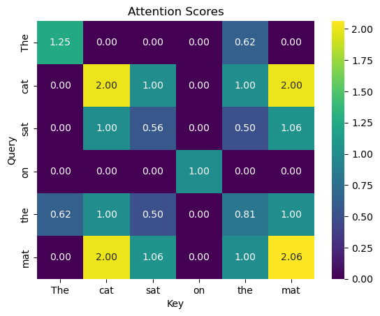
As you can see, we’re getting matches across all words in our sequence with “cat” and “mat” receiving very high attention. Our players found each other!
Triangular Masking in Self-Attention
There is one wrinkle with this attention-matrix: words earlier in the sequence can look “forward in time” to words that appear later. This is fine for some applications, but if we want a model to predict the next word based on previous words, we can’t train the model on scenarios where it has access to the full document.
In our case, we don’t want “cat” to attend to “mat” because that word is later in the sentence. For this, we use a mechanism called triangular masking which blanks out all later-occuring words.
Imagine a game of “Inkognito” where you can only exchange information with every player that came before you. Similarly, in language processing, especially in tasks like text generation, it’s important that the model only considers the words it has seen so far, not the words that are yet to come.
# Applying triangular masking
mask = np.tril(np.ones_like(attention_scores))  # Lower triangular matrix
masked_attention_scores = attention_scores * mask

# Visualize the attention scores
sns.heatmap(masked_attention_scores, annot=True, cmap='viridis', fmt=".2f")
plt.title("Attention Scores")
plt.xlabel("Key")
plt.ylabel("Query")
plt.show()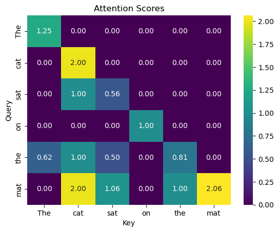
Now, every word only attends to words that preceded it.
Normalizing the attention scores
For keeping things nice and scaled, it’s also a good idea to normalize every row. We don’t want players to find each other easier just by shouting louder than others.
# Applying softmax for normalization
normalized_attention_scores = masked_attention_scores.divide(masked_attention_scores.sum(1), 0)

# Visualize the normalized attention scores
sns.heatmap(normalized_attention_scores, annot=True, cmap='viridis', fmt=".2f")
plt.title("Normalized Attention Scores")
plt.xlabel("Key")
plt.ylabel("Query")
plt.show()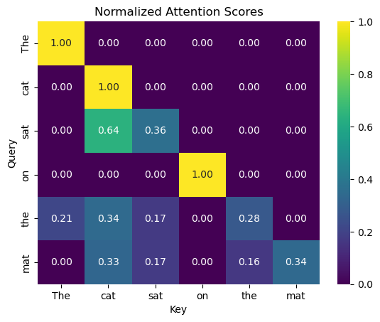
When coding things up, usually a softmax is used instead of the explicit normalization.
Exchange of information
Now that our players have found each other, they next exchange their secret information: their values. This is done by mapping words to values via a third matrix W_v. We basically allow for a linear transformation of the inputs.
W_v = np.random.randn(*input_sequence.shape)
values = input_sequence @ W_v.T
In the final step, we apply the attention-weighting to the values to come up with a new representation for each word. This new representation is an attention-weighted average of the (value-transformed) words that preceded this word. You can think of this as now the players have all found each other and exchanged their secrets to yield the complete information shared across all players.
output = normalized_attention_scores @ values
output| 0 | 1 | 2 | 3 | 4 | 5 | |
|---|---|---|---|---|---|---|
| The | -0.964624 | -0.524278 | 1.188478 | 0.793799 | -1.902606 | -1.350984 |
| cat | 1.689457 | 0.492961 | -1.076842 | -0.444506 | -0.178372 | -0.186791 |
| sat | 0.848836 | -0.013991 | -0.749261 | -0.439678 | -0.118622 | -0.157566 |
| on | 0.275485 | -0.011855 | 0.770311 | 0.064108 | 0.749518 | -0.931713 |
| the | 0.360249 | -0.103849 | -0.126685 | -0.007499 | -0.755438 | -0.581679 |
| mat | 0.565891 | -0.225550 | -0.608965 | -0.411417 | -0.264478 | -0.271858 |
And that’s in essence how the self-attention mechanism underlying LLMs like GPT works. In practice, you would not just have a single attention mechanism (so-called head), but many in parallel, so that a single word can interact with different words. You can think of this as players not just having to find each other according to one set of rules, but various other players according to different sets of rules simultaneously.
In reality, GPT also does not use full words but rather word chunks (i.e. tokens). You might have also noticed that this encoding is permutation-invariant – we get the same results even if we switch the order of the words. This is solved by an additional mechanism called positional encoding.
Computational considerations
One key reason of why self-attention is so powerful is its computational properties. All we did above was perform matrix multiplications. Recurrent neural nets like LSTMs have the big draw-down of not being parallelizable because you can only feed data in sequentially to progressively build up state.
Beyond Self-Attention: Enhancing Large Language Models
While self-attention is a critical component of modern LLMs like GPT, it’s just one piece of a larger puzzle. These models leverage a range of techniques to improve learning efficiency, accuracy, and generalization. Let’s explore some of these key techniques:
Layer Normalization
Layer Normalization is akin to a player in “Inkognito” taking a moment to organize their thoughts and clues before making a move. In neural networks, it’s about standardizing the inputs to each layer within a network. By normalizing the inputs across features, layer normalization stabilizes the learning process and helps in faster convergence.
# Example of layer normalization in pseudocode, ignoring learnable parameters alpha and beta
normalized_output = (input - mean(input)) / sqrt(var(input))
Skip Connections (Residual Connections)
Skip connections, or residual connections, are like shortcuts in the game of “Inkognito” that allow players to revisit previous clues quickly. In neural networks, they enable the output of one layer to “skip” over some layers and be added to the output of a later layer. This helps in mitigating the vanishing gradient problem and allows for deeper networks by facilitating smoother gradient flow.
# Example of a skip connection in pseudocode
output = activation(input + previous_layer_output)
Dropout
Dropout is a technique that can be likened to adding an element of unpredictability in “Inkognito,” where players might occasionally withhold certain information. This makes players more robust because they learn how to handle missing information. In neural networks, dropout randomly turns off a proportion of neurons during training, which helps prevent overfitting and encourages the network to learn more robust features.
# Example of dropout in pseudocode
dropout_output = randomly_disable_neurons(input, dropout_rate)
Other Techniques
Modern LLMs often incorporate additional techniques, such as attention dropout (adding randomness to the attention mechanism), varying learning rates, and specialized activation functions. Each of these contributes to the model’s ability to learn effectively and generalize well.
Deep Nets
Self-attention, plus all these techniques combined with dense feed-forward layers and non-linear activation functions make up a single layer. We then stack many of these layers on top of each other - the more the merrier.
The Symphony of Techniques in LLMs
Just as winning “Inkognito” requires a blend of strategies, skills, and a bit of luck, crafting effective LLMs like GPT involves harmonizing various neural network techniques. Self-attention provides the mechanism to understand and contextualize data, while layer normalization, skip connections, dropout, and other methods ensure that the learning process is stable, efficient, and robust.
Conclusion
To sum up, self-attention consists of 3 key mechanisms that are combined in a simple yet clever manner: * Keys provide a (learnable) signature for each word by which other words can find it. Its saying “this is what I am”. * Queries represent the other side of that search and communicate what signature that word is seeking. Its saying “this is what I’m looking for”. * Keys are matched to queries to provide the attention scores. * We then use the attention scores to compute a weighted-sum of the values. Values are a linear transformation of the inputs and represent the information content.
Through this mechanism, words can get mixed up with other words that occur elsewhere in the sequence and build richer representations that take long-range context into account.
Hopefully this explanation provided a more intuitive understanding. For me, self-attention was the most difficult concept to grok, the other stuff is more a bag of tricks that works well in practice.
But even after getting a more intuitive understanding of how a model like GPT works, and factoring in the enormous scale of the data and model, I’m in awe as to how a few matrix multiplications can produce outputs that appear very intelligent. The answer must lie in these higher-order representations that these networks build up.
References
- The most useful resource I found is this tutorial by Andrej Karpathy “Building a GPT from scratch” https://www.youtube.com/watch?v=kCc8FmEb1nY